I have kept a blog on this site for quite some years. It was mostly about using open source GIS tools. Although I enjoyed writing the posts, other things became more important, and I haven’t written a post for quite a while.
However, I am planning to pick it up again. But not on this site. Although it has served me well, I have decided to go for a different solution. I will use Hugo together with Blogdown to write my posts. You’ll find them on Ecodiv.earth. Hope to see you there!
Population density maps have multiple implications, e.g., to help relief agencies to better plan where they are needed most in case of disaster and in demographic, economic and environmental research. However, in large parts of the world, it has always been difficult to produce accurate and consistent population (density) maps based on existing census data.
Three well known initiatives to produce consistent and high resolution population (density) maps are the Gridded Population of the World (GPW), the Global Rural-Urban Mapping Project (GRUMP) and the Worldpop data. The first two, both published by SEDAC, come at a resolution of 30 arc seconds (approximately 1 km at the equator). The Worldpop data set comes at a higher resolution of 3 arc seconds (approximately 100 m at the equator) (Tatem 2017). This was achieved by disaggregating census data using machine learning algorithms with remote sensing data and other data sources (Stevens et al., 2015).
For an overview of the differences between different data sets, including the three mentioned above, check out the Popgrid Viewer by SEDAC. It provides a comparison of key characteristics of each data set. In addition, it provides an online viewer in which you can compare the maps side by side.
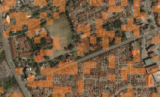
Recently, an even higher resolution population density map has been published by Facebook in collaboration with other parties. It is based on a mixture of machine learning techniques, high-resolution satellite imagery population data and OpenStreetMap (OSM). The result is a population density map at the impressive resolution of 1 arc seconds (approx. 30 meter at the equator). That is at the scale of a (large) building (!).
Population density in a neighborhood of Nairobi, Kenya.
Population densities on the slopes of Mount Kenya
Population density at the neighborhood level
The images in the gallery above show that you should not expect to be able to identify individual houses in high density urban areas. On the other hand, it gives a pretty good idea of where people live on more remote areas on the slope of Mount Kenya. All in all, this map seems to capture the distribution of people across the landscape more accurately and at higher resolution than other maps mentioned earlier.
Of course, it is not only about spatial resolution. It is also about the accuracy of the population density estimates. In that respect, it is important to remember that the density estimates depend on the accuracy of the underlying census data, and that this data is largely the same as used in the maps mentioned earlier. On the other hand, at resolution of this map, you can actually start to compare population density estimates with the actual number of people in your block, and thus validate the map at a very local, sub-neighborhood level.
After almost 1 year of development the GRASS Development team has released the new stable release GRASS GIS 7.6.0. A big thanks to all developers for their work and dedication!
There is a lot to like, including further improvements to the user experience and new useful additional functionalities to modules. I, for example am curious to try out the new raster map type, the GRASS virtual raster (VRT). This is a virtual mosaic of a list of input raster maps.
But I would say, head over to the overview page where you can read more about the new features in the 7.6 release series: new features in GRASS GIS 7.6. Or update GRASS and check out yourself.
For those who missed it, a new update release GRASS GIS 7.4.4 is available since the 4th of January. It mainly brings bugfixes, but it also includes an important new function, the module r.mapcalc.simple. This module is especially important for a better integration with QGIS. It therefore has already been dubbed the “QGIS friendship” release :).
I am currently working on some exercises for which I need data about municipalities in the Netherlands. A good place to look for such data is the CBS (Dutch Central Bureau of Statistics). One data layer is vector layers of the dutch municipalities and neighborhoods, which include demographic data.
One of the first things I normally do when exploring new data is to look at the distribution of the data. For example by creating a histogram using the d.vect.colhist addon (see my earlier post). But what if I want to compare the distribution of different groups or samples? In such a case I find boxplots more convenient. However, there is no tool in GRASS GIS to create boxplots, so I had a look at the d.vect.colhist addon code and adapted the code to create boxplots instead of histograms.
An example
Let’s for example look at the average population densities of the municipalities.
The average population density (number of inhabitants / km2) per municipality in 2017. Source: CBS.
What if I want to compare the distribution of the average population density per provinces Dutch provinces? You can install the addon (see the end of this post) and run d.vect.colbp on the command line or the console. This will open a window with different tabs.
In the first tab, you can define a column in the attribute table to plot (here BEV_DICHTH, which is the column with the population density) and a column that will be used to group the data (here provincie, which gives the names of the provinces the municipality belongs to). As you can see in the screenshot above, you have a few options to change the plot (layout). In this case, I choose to rotate the x-axis labels so they do not overlap. The resulting plot looks like:
The distribution of the average population densities of the Dutch municipalities per province.
You can of course also use the command line. In this case I will plot the boxplots horizontally using the ‘h flag’.
The distribution of the average population densities of the Dutch municipalities per province.
The add-on does not provide further options to change the appearance of the plot, as the main idea is to use this for quick exploration of your data, similar to the other plotting tools in GRASS GIS. However, you can save the plot as a svg file, and further edit it in e.g., Inkscape.
You can install the addon using the g.extension to install the addon:
g.extension d.vect.colbp
Any feedback will be most welcome. If you try it out and run into problems, please let me know (suggestions for improvements are of course also welcome).
GRASS GIS has convenient tools to draw histograms of raster values. As similar tool to draw a histogram of values in a vector attribute table lacks. But you can easily add this functionality by installing the d.vect.colhist addon by Moritz Lennert. Read this short post on Ecodiv.earth tutorials.
A great source of information about GRASS GIS is the GRASS Wiki. One example is this list with GRASS GIS Jupyter notebooks which was just added by Markus Neteler (no introduction needed I guess). There are some really nice tutorials there, which alone is reason enough to check out this list. Continue reading “GRASS GIS Jupyter notebooks”→
A common technique to estimate the accuracy of a predictive model is k-fold cross-validation. In k-fold cross-validation, the original sample is randomly partitioned into a number of sub-samples with an approximately equal number of records. Of these sub-samples, a single sub-sample is retained as the validation data for testing the model, and the remaining sub-samples are combined to be used as training data. The cross-validation process is then repeated as many times as there are sub-samples, with each of the sub-samples used exactly once as the validation data (Table 1).
Table 1. Illustration of data partitioning in a 4-fold cross-validation, with training data used to train the model, and test data to validate the model.
The k evaluation results can then be averaged (or otherwise combined) to produce a single estimation. The advantage of this method is that all observations are used for both training and validation, and each observation is used for validation exactly once.
Functions for modelling and machine learning in e.g., R and Python’s Scikit-learn often contain build-in cross-validation routines. But it is also fairly easy to build such a routine yourself. This tutorial shows how one can easily build a k-fold cross-validation routine in GRASS GIS, e.g., to evaluate the predictive performance of two interpolation techniques, the inverse Distance Weighting and bilinear spline interpolation.
Figure 1. A) Elevation map of North Carolina. B) Elevation estimation based on inverse distance weighting interpolation of the elevation at 150 random sample points. C) Residue map with the differences between A and B. D) Relative differences between A and B, computed as (A-B)/A. Map C and D are overlaid with the 150 sample locations.